5 Tips and Tricks

• Spell check functionality in RStudio

Although often overlooked, RStudio can check your spelling

• New line for each sentence

5.1 Global chunk options

It can be useful to set chunk options globally for all (following) chunks to avoid retyping or copy-and-pasting

# Save all plots as 600 DPI TIFF-files
knitr::opts_chunk$set(dev = "tiff", dpi = 600)

# Do not evaluate subsequent chunks (debugging or fine-tuning)
knitr::opts_chunk$set(eval = FALSE)

See the knitr chunk options and package options for an overview of settings

5.2 Meaningful chunk names

…

5.3 Text references

Because papaja extends bookdown you can use text references in any papaja document. A text reference consists of a unique label—defined as (ref:unique-label) somewhere in the body of the document (not inside a code chunk)—and the text that the label stands in for. Text references must be defined in a separate single-line paragraph with empty lines above and below:

(ref:my-caption) This is a caption for my table.

The definition of a text reference must be on a single line and should not end with a white space. Hence, the following will not work as expected

(ref:my-caption) 
This is a caption for my table.

Using text references for table and figure captions has several advantages:

1. Markdown and \(\LaTeX\) syntax is not well supported in chunk options, such as fig.cap, or elsewhere inside a code chunk, e.g., in the caption argument of apa_table(). Specifically, Markdown formatting and citation syntax are ignored (rendered as-is) and, for example, \ and _ must be escaped to prevent errors in either R or \(\LaTeX\). None of these limitations apply to text references.
2. Long captions can impair the readability of the document when they are part of chunk options or R code.
3. knitr considers modifications of the text in fig.cap as changes to the code chunk and hence may invalidate the cache of a chunk. As a consequence cached results of the code chunk need to be recomputed. Changes to the text of a text reference do not invalidate the cached computations.
4. It’s straight forward to include inline code chunks in text references.

Text references can be used to duplicate information throughout the document. Consider the following example.

(ref:aesthetics) Points represent conditions means, error bars represent 955% confidence intervals.

(ref:caption1) An interesting plot.

```{r fig.cap = paste("(ref:caption1)", "(ref:aesthetics)")}
apa_beeplot(data = npk, id = "block", dv = "yield", factors = "N")
```

(ref:caption2) Another interesting plot.

```{r fig.cap = paste("(ref:caption2)", "(ref:aesthetics)")}
apa_beeplot(data = npk, id = "block", dv = "yield", factors = "N")
```

The resulting figure caption combines the two text references, Figure 5.1.

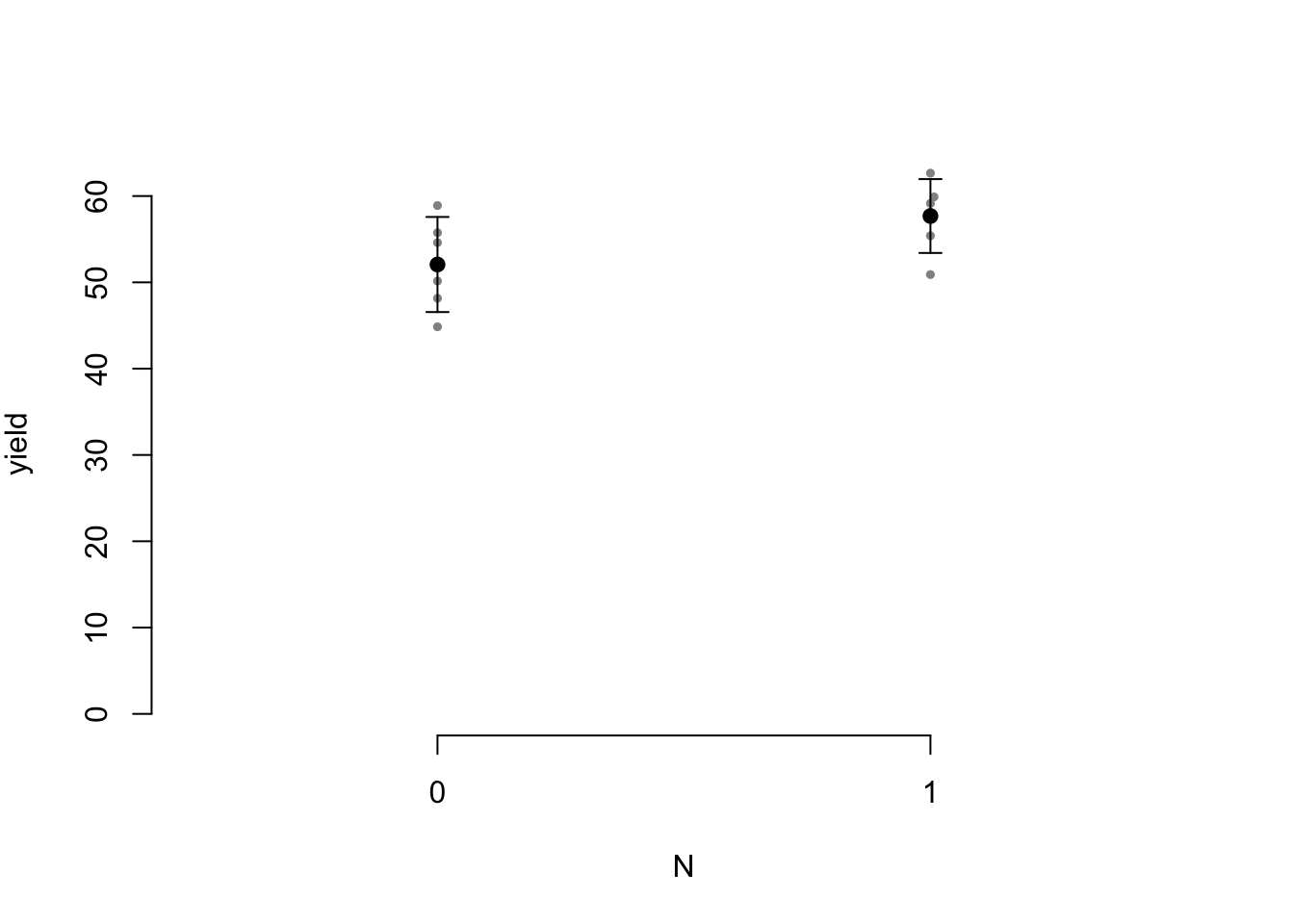
Figure 5.1: An interesting plot. Points represent conditions means, error bars represent 955% confidence intervals.

Because the information about what points and error bars represent is repeated using a text reference, and not by literal repetition throughout the document, it’s easy to correct the typo (955% confidence intervals) and be sure that it is corrected in every instance.

5.4 Useful RStudio Addins

• citr: Insert Markdown Citations
• remedy: Keyboard shortcuts for Markdown formatting
• splitChunk: Split R Markdown code chunks
• gramr: Write-good linter
• wordcount: Word counts and readability statistics

Set up keyboard shortcuts via
Tools > Modify keyboard shortcuts

Suggested keyboard shortcuts

Package	Addin	Keyboard shortcut
citr	Insert citation	Shift + Alt+R
wordcount	Word count	Shift + Alt+C
splitChunk	Chunk split	Shift + Alt+S
remedy	Bold	Shift + Alt+B
	Italic	Shift + Alt+I
	Backtick	Shift + Alt+P
	URL	Shift + Alt+U

• statcheck: Extract Statistics from Articles and Recompute p Values
• retractcheck: Check DOIs in a paper for retractions

5.5 Reproducible software environments

To ensure mid- to long-term computational reproducibility, we highly recommend conserving the software environment used to write a manuscript (e.g. R and all R packages) either in a software container or a virutal machine. This helps to avoid code rot (that is, your R code breaking because of updates to, for example, R or any R package) and ensures you can reproduce your analysis in the years to come. For a brief primer on containers and virtual machines see the supplementary material by Klein et al. (2018).

5.5.1 Docker

Docker is probably the most widely used containerization approach. Docker containers are similar to virtual machines: insulated software environments (system libraries, R, R packages, RStudio, LaTeX, LaTeX packages, etc.) that run inside your host system. Docker works on most operating systems and is widely used, free, and open source. It just requires some disk space. For a concise hands-on introduction see the ROpenSci Docker tutorial; a more detailed introduction is available from the Docker project. Docker containers are configured using so-called Docker files that act as a recipe for the software environment. With the Docker file, anyone can automatically recreate the software environment that you used and rerun your analysis. As a starting point for your container you can build on the following Docker file, which sets up everything that is needed for creating a manuscript with papaja—including an instance of RStudio that you can access through your browser:

# Look up available R versions at https://github.com/rocker-org/rocker-versioned/tree/master/verse

FROM rocker/verse:3.6.3

# Install papaja dependencies
RUN apt-get update \
    && apt-get install -y --no-install-recommends \
    libgsl0-dev \
    libnlopt-dev

RUN install2.r --error \
    --skipinstalled \
    --deps TRUE \
    rmdfiltr

# Required by broom -- obsolete once newer versions are available from MRAN
RUN Rscript -e "remotes::install_version('rlang', '0.4.7', repos = 'http://cran.us.r-project.org', upgrade = FALSE, Ncpus = 3)"
RUN Rscript -e "remotes::install_version('tidyselect', '1.1.0', repos = 'http://cran.us.r-project.org', upgrade = FALSE, Ncpus = 3)"
RUN Rscript -e "remotes::install_version('vctrs', '0.3.2', repos = 'http://cran.us.r-project.org', upgrade = FALSE, Ncpus = 3)"
RUN Rscript -e "remotes::install_version('dplyr', '1.0.0', repos = 'http://cran.us.r-project.org', upgrade = FALSE, Ncpus = 3)"

# Latest papaja development version
RUN Rscript -e "remotes::install_github('crsh/papaja',  quick = FALSE, build = TRUE, dependencies = c('Depends', 'Imports'), Ncpus = 3, upgrade = FALSE)"

Place this Docker file in your project directory alongside the following bash script (for MacOS or Linux):

#!/bin/sh

docker build \
    --build-arg RSTUDIO_VERSION=1.3.1093 \
    -t container-name .

docker run -d \
    -p 8787:8787 \
    -e DISABLE_AUTH=true \
    -e ROOT=TRUE \
    -v $(pwd):/home/rstudio \
    container-name

sleep 1

open http://$(ipconfig getifaddr en0):8787

Execute this script in your project directory to set up and run the container. This script will take a little while to finish the first time around (it downloads the base container and installs all needed R packages), but should be fast the next time. Finally, a browser window with an instance of RStudio should open and all files from you project directory should be shared between your container and the host system. You can work in that RStudio instance in your browser just as you usually would.

Note that whenever you install an R package interactively (i.e., via the GUI or install.packages()) they will be lost once you stop the container. While this may seem inconvenient, it ensures that your Docker file (that is your recipe) is complete.

To permanently install new R packages in your container, add them to the Docker file. For example,

RUN install2.r --error \
    --skipinstalled \
    --deps TRUE \
    rmdfiltr
    afex
    emmeans

Note that all R packages are installed from MRAN, which serves packages as they were available from CRAN on a particular date in the past. For the rocker images used here this date is the last day the desired version of R was the most recent release, see the rocker version information for details.

If the installation of the required R packages takes a long time, it may help to install the packages and their dependencies in parallel. To install packages using three cores in parallel, add --ncpus 3 \ to the above RUN instructions.

5.5.2 CodeOcean

CodeOcean is a commercial service that builds on Docker, facilitates setting up and sharing containers, and lets you run computations in the cloud. In case you prefer CodeOcean over plain Docker, you may be interested in the minimal papaja example capsule that CodeOcean’s Seth Green has kindly prepared. If you want to use papaja in your next CodeOcean project, you may use this capsule as a starting point.

5.6 RStudio

1. Document outline

RStudio provides a handy document outline view

5.7 Splitting an R Markdown document

Some authors may prefer to split long manuscripts into multiple component files for better clarity. There are two basic strategies to split R Markdown documents that can be combined or used in isolation: sourcing R scripts and splitting the R Markdown document. If the R Markdown document contains a lot of code, it may be helpful to disincorporate parts of the code, such as reading, merging, restructuring, and relabeling data files. The R scripts can then be executed at the respective section of the document using source().

Some authors may prefer to split long manuscripts into a master or parent document and multiple children. The master document, for example, consists of the YAML front matter and includes the children, which are themselves R Markdown documents without a YAML front matter. To include a child document, insert an empty chunk and provide the path to the R Markdown document in the chunk option child.

It may be preferable to split long documents into multiple files

```{r child = "introduction.Rmd"}
```

```{r child = "method.Rmd"}
```

```{r child = "results.Rmd"}
```

```{r child = "discussion.Rmd"}
```

Search all files with Ctrl + Shift+F

5.8 Best practices

1. Load all R packages in the first code chunk
   • Never include install.packages()
2. Set a seed for random number generators
   (e.g., set.seed())
3. Never use setwd()!
4. Use relative paths or load files from a permanent location
5. Use meaningful chunk names
6. Keep R code close to the corresponding prose
7. Document R and R-package versions
   (e.g., devtools::session_info())
8. Try to ensure you can knit without errors before going home

5.9 Troubleshooting

As detailed in Document compilation, rendering a papaja document involves several software packages. This layered software design grants the package its capabilities but it comes at a cost: When compilation of a papaja-document throws an error it may not be immediately obvious to an inexperienced user, which part of the process failed. However, the error message usually give some indication which portion of the process errored:

1. Parsing of the YAML front matter
   • Error in yaml::yaml.load(enc2utf8(string), ...) :
2. R code execution
   • Error: Object 'x' not found.
3. bookdown adds cross- and text-references
   • No error messages; look for in text
4. pandoc document conversion
   • Error: pandoc document conversion failed with error 1
   • Error running filter /path/to/filter/filter.lua
5. pandoc-citeproc reference generation
   • pandoc-citeproc: Cannot decode byte '\xfc'
   • pandoc-citeproc: reference X not found, shows up as ??? in text
6. \(\LaTeX\) PDF generation
   • ! Missing $ inserted

It is often helpful to search the internet for the error messages or portions thereof. Many times others will have encountered the same problem and may have documented their solution. In the following we provide some general advice.

5.9.1 YAML

TBD

Double check indentation and white space.

5.9.2 R

Error messages generated by R unfortunately do not provide the exact line that has errored. The reported line number indicates the first line of R code chunk that contains the erroneous code.

Fixing bugs in R Markdown documents can be challenging because the code is run in a new non-interactive R session. This makes it a little harder to play around to pinpoint what’s causing the problem. Hence, do your best to recreate the problem in your interactive session:

1. Restart R (Session > Restart R or
   Ctrl + Shift + F10 in RStudio)
2. Compare the working directories (e.g., use getwd() in the console and in a code chunk of your knitted document)
3. Run every chunk individually until you get the error

If you can’t reproduce the problem in your interactive R session, there must be some difference between it and the R environment of your document. Once you identify that difference you will often know what is causing the problem. If you don’t you at least can now recreate the problem in your interactive R session and start debugging. To learn more about debugging techniques refer to Advanced R (Wickham, 2019).

5.9.3 bookdown

TBD

Don’t use _ in chunk names!

5.9.4 pandoc

TBD

Report errors with papaja Lua filters at https://github.com/crsh/papaja/issues

5.9.5 \(\LaTeX\)

TBD

Inspect the log file.

Comments and Questions

Icons by Icons8